Search results
Jump to navigation
Jump to search
Page title matches
File:Figure C-11.jpg (1,052 × 1,966 (263 KB)) - 20:24, 6 April 2016
File:Figure C-9.jpg (1,098 × 2,008 (231 KB)) - 20:26, 6 April 2016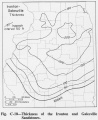
File:Figure C-10.jpg (1,076 × 1,313 (204 KB)) - 20:24, 6 April 2016
File:Figure C-12.jpg (1,051 × 1,952 (298 KB)) - 20:23, 6 April 2016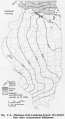
File:Figure C-2.jpg (1,093 × 1,998 (321 KB)) - 20:18, 6 April 2016
File:Figure C-13.jpg (1,050 × 1,987 (293 KB)) - 20:21, 6 April 2016
File:Figure C-3.jpg (1,086 × 3,012 (377 KB)) - 17:19, 25 May 2016
File:Figure C-1A.jpg (1,917 × 1,187 (1,023 KB)) - 20:18, 6 April 2016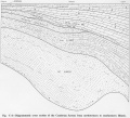
File:Figure C-4.jpg (2,113 × 1,914 (585 KB)) - 20:18, 6 April 2016
File:Figure C-1B.jpg (1,509 × 2,000 (1.18 MB)) - 20:18, 6 April 2016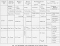
File:Figure C-5.jpg (2,209 × 1,696 (388 KB)) - 20:17, 6 April 2016
File:Figure C-1C.jpg (1,482 × 2,000 (788 KB)) - 20:19, 6 April 2016
File:Figure C-6.jpg (1,058 × 1,973 (233 KB)) - 20:26, 6 April 2016
File:Figure C-1D.jpg (1,387 × 2,000 (776 KB)) - 20:19, 6 April 2016
File:Figure C-7.jpg (1,081 × 1,991 (261 KB)) - 20:22, 6 April 2016
File:Figure C-8.jpg (1,056 × 1,967 (260 KB)) - 20:26, 6 April 2016
File:Figure C-3 imagemap.jpg (350 × 971 (100 KB)) - 15:08, 30 November 2016


Page text matches
- Figure D-3A.jpg|{{file:Figure D-3A.jpg}} Figure D-3B.jpg|{{file:Figure D-3B.jpg}}4 KB (626 words) - 20:53, 5 January 2017
- Figure D-3A.jpg|{{file:Figure D-3A.jpg}} Figure D-3B.jpg|{{file:Figure D-3B.jpg}}5 KB (698 words) - 21:35, 6 January 2017
- Figure D-3C.jpg|{{file:Figure D-3C.jpg}}4 KB (561 words) - 22:03, 6 January 2017
- Figure P-2.jpg|{{file:Figure P-2.jpg}} Figure P-5.jpg|{{file:Figure P-5.jpg}}5 KB (747 words) - 22:02, 24 January 2017
- Figure D-3C.jpg|{{file:Figure D-3C.jpg}}5 KB (632 words) - 17:46, 11 January 2017
File:C605-Figure-37.jpg |File name=C605-Figure-37.jpg |image_no=Figure 37(1,535 × 1,872 (579 KB)) - 19:29, 23 August 2023
File:C605-Figure-05a.jpg |File name=C605-Figure-05a.jpg |image_no=Figure 5a(1,905 × 1,774 (937 KB)) - 15:43, 17 August 2023
File:C605-Figure-05b.jpg |File name=C605-Figure-05b.jpg |image_no=Figure 5b(2,000 × 2,085 (1.13 MB)) - 15:43, 17 August 2023
File:104-Figure 9.jpg Figure 9 -- History of the litho-stratigraphic classification of the Mason Group d(1,527 × 2,000 (345 KB)) - 16:24, 19 April 2016
File:Penn carbondale 4-44.jpg |Caption=Figure 4-44. Graphic log of core (partial) from Freeman United Coal Mining Compan(1,266 × 3,627 (625 KB)) - 19:19, 23 December 2020- Figure S-2A.jpg|{{file:Figure S-2A.jpg}} Figure S-2B.jpg|{{file:Figure S-2B.jpg}}13 KB (2,005 words) - 19:56, 4 January 2017
- Figure K-1A.jpg|{{file:Figure K-1A.jpg}} Figure K-1B.jpg|{{file:Figure K-1B.jpg}}3 KB (381 words) - 05:20, 28 December 2016
- Figure S-2A.jpg|{{file:Figure S-2A.jpg}} Figure S-2B.jpg|{{file:Figure S-2B.jpg}}14 KB (2,077 words) - 18:14, 11 January 2017
- Figure K-1A.jpg|{{file:Figure K-1A.jpg}} Figure K-1B.jpg|{{file:Figure K-1B.jpg}}3 KB (459 words) - 20:27, 12 January 2017
- Figure 14.jpg|{{file:Figure 14.jpg}} Figure P-3D.jpg|{{file:Figure P-3D.jpg}}3 KB (482 words) - 22:16, 19 January 2017
- ...lt or overlying beds. Its spatial relations are shown diagrammatically in figure 8. The geographic distribution of the member is shown in figure 6.2 KB (318 words) - 22:21, 3 January 2017
- Figure P-3B.jpg|{{file:Figure P-3B.jpg}}2 KB (268 words) - 16:14, 25 January 2017
- Figure P-2.jpg|{{file:Figure P-2.jpg}}2 KB (252 words) - 22:20, 19 January 2017
- Figure C-1A.jpg|{{file:Figure C-1A.jpg}} Figure C-1B.jpg|{{file:Figure C-1B.jpg}}4 KB (585 words) - 16:52, 28 November 2016
- ...shown in figure 6, and the spatial relations are shown diagrammatically in figure 8.2 KB (299 words) - 20:56, 12 January 2017
- Figure 14.jpg|{{file:Figure 14.jpg}} Figure P-3D.jpg|{{file:Figure P-3D.jpg}}4 KB (561 words) - 22:48, 19 January 2017
- Figure O-2B.jpg|{{file:Figure O-2B.jpg}} Figure O-2C.jpg|{{file:Figure O-2C.jpg}}4 KB (525 words) - 17:37, 8 December 2016
- Figure D-6.jpg|{{file:Figure D-6.jpg}}2 KB (341 words) - 21:50, 6 January 2017
- Figure P-2.jpg|{{file:Figure P-2.jpg}}3 KB (401 words) - 20:36, 20 January 2017
- Figure P-2.jpg|{{file:Figure P-2.jpg}}3 KB (433 words) - 17:31, 24 January 2017
- Figure O-2B.jpg|{{file:Figure O-2B.jpg}}2 KB (288 words) - 19:11, 8 December 2016
- Figure O-2B.jpg|{{file:Figure O-2B.jpg}}2 KB (285 words) - 17:25, 13 December 2016
- Figure O-2B.jpg|{{file:Figure O-2B.jpg}}2 KB (292 words) - 18:32, 8 December 2016
- Figure O-2D.jpg|{{file:Figure O-2D.jpg}} Figure O-2F.jpg|{{file:Figure O-2F.jpg}}3 KB (494 words) - 22:29, 14 December 2016
- Figure P-2.jpg|{{file:Figure P-2.jpg}} Figure P-5.jpg|{{file:Figure P-5.jpg}}3 KB (462 words) - 21:40, 2 March 2018
- Figure O-2B.jpg|{{file:Figure O-2B.jpg}}2 KB (288 words) - 17:50, 13 December 2016
- Figure P-2.jpg|{{file:Figure P-2.jpg}}3 KB (330 words) - 23:03, 19 January 2017
- Figure P-3B.jpg|{{file:Figure P-3B.jpg}}2 KB (352 words) - 16:03, 25 January 2017
- Figure O-2B.jpg|{{file:Figure O-2B.jpg}} Figure O-2C.jpg|{{file:Figure O-2C.jpg}}4 KB (600 words) - 16:44, 12 January 2017
- Figure P-3B.jpg|{{file:Figure P-3B.jpg}}3 KB (344 words) - 17:28, 25 January 2017
- Figure C-1A.jpg|{{file:Figure C-1A.jpg}} Figure C-1B.jpg|{{file:Figure C-1B.jpg}}5 KB (657 words) - 20:50, 11 January 2017
- Figure O-2B.jpg|{{file:Figure O-2B.jpg}}2 KB (292 words) - 18:20, 8 December 2016
- Figure O-2B.jpg|{{file:Figure O-2B.jpg}}2 KB (306 words) - 17:48, 13 December 2016
- Figure C-1C.jpg|{{file:Figure C-1C.jpg}}4 KB (541 words) - 21:00, 28 November 2016
- Figure O-2D.jpg|{{file:Figure O-2D.jpg}} Figure O-2F.jpg|{{file:Figure O-2F.jpg}}4 KB (568 words) - 17:58, 12 January 2017
- ...lt or overlying beds. Its spatial relations are shown diagrammatically in figure 8. The geographic distribution of the member is shown in figure 6.3 KB (385 words) - 20:43, 12 January 2017
- Figure P-2.jpg|{{file:Figure P-2.jpg}} Figure P-16.jpg|{{file:Figure P-16.jpg}}4 KB (523 words) - 16:35, 20 January 2017
- Figure P-2.jpg|{{file:Figure P-2.jpg}} Figure P-15.jpg|{{file:Figure P-15.jpg}}4 KB (503 words) - 17:57, 23 January 2017
- ...shown in figure 6, and the spatial relations are shown diagrammatically in figure 8.3 KB (349 words) - 21:10, 12 January 2017
- Figure C-1D.jpg|{{file:Figure C-1D.jpg}}4 KB (575 words) - 18:13, 28 November 2016
- Figure O-2B.jpg|{{file:Figure O-2B.jpg}}3 KB (366 words) - 16:56, 12 January 2017
- Figure P-2.jpg|{{file:Figure P-2.jpg}}3 KB (460 words) - 21:16, 27 January 2017
- Figure O-2B.jpg|{{file:Figure O-2B.jpg}}3 KB (369 words) - 16:55, 12 January 2017
- Figure O-2B.jpg|{{file:Figure O-2B.jpg}}3 KB (373 words) - 16:49, 12 January 2017
- Figure O-2B.jpg|{{file:Figure O-2B.jpg}}3 KB (369 words) - 16:59, 12 January 2017
- Figure O-2B.jpg|{{file:Figure O-2B.jpg}}3 KB (375 words) - 16:46, 12 January 2017
- Figure O-2B.jpg|{{file:Figure O-2B.jpg}}3 KB (386 words) - 16:58, 12 January 2017
- Figure O-2B.jpg|{{file:Figure O-2B.jpg}} Figure O-2C.jpg|{{file:Figure O-2C.jpg}}5 KB (726 words) - 16:41, 12 January 2017
- Figure D-6.jpg|{{file:Figure D-6.jpg}}3 KB (425 words) - 17:33, 11 January 2017
- Figure P-2.jpg|{{file:Figure P-2.jpg}}3 KB (478 words) - 22:34, 20 January 2017
- Figure M-1B.jpg|{{file:Figure M-1B.jpg}} Figure M-1D.jpg|{{file:Figure M-1D.jpg}}4 KB (560 words) - 15:25, 22 October 2019
- Figure P-2.jpg|{{file:Figure P-2.jpg}}4 KB (509 words) - 19:49, 24 January 2017
- Figure P-2.jpg|{{file:Figure P-2.jpg}} Figure P-14.jpg|{{file:Figure P-14.jpg}}4 KB (541 words) - 16:53, 24 January 2017
- ...the Winnebago to adjacent stratigraphic units is shown diagrammatically in figure 8. ...ic distribution of the formation at the surface is indicated on the map in figure 6.5 KB (697 words) - 20:55, 12 January 2017
- Figure M-1B.jpg|{{file:Figure M-1B.jpg}} Figure M-1E.jpg|{{file:Figure M-1E.jpg}}4 KB (593 words) - 22:59, 17 January 2017
- Figure P-3B.jpg|{{file:Figure P-3B.jpg}}3 KB (424 words) - 17:25, 25 January 2017
- Figure K-1A.jpg|{{file:Figure K-1A.jpg}}3 KB (506 words) - 17:34, 21 November 2016
- Figure M-1A.jpg|{{file:Figure M-1A.jpg}} Figure M-1B.jpg|{{file:Figure M-1B.jpg}}9 KB (1,331 words) - 16:04, 10 January 2017
- Figure P-3B.jpg|{{file:Figure P-3B.jpg}}3 KB (355 words) - 23:06, 24 January 2017
- Figure P-2.jpg|{{file:Figure P-2.jpg}}3 KB (346 words) - 17:19, 25 January 2017
- Figure P-2.jpg|{{file:Figure P-2.jpg}}3 KB (399 words) - 18:34, 27 January 2017
- Figure O-2D.jpg|{{file:Figure O-2D.jpg}}3 KB (516 words) - 22:29, 19 December 2016
- Figure M-1B.jpg|{{file:Figure M-1B.jpg}} Figure M-1E.jpg|{{file:Figure M-1E.jpg}}5 KB (728 words) - 15:19, 22 October 2019
- Figure O-2B.jpg|{{file:Figure O-2B.jpg}} Figure O-2C.jpg|{{file:Figure O-2C.jpg}}5 KB (788 words) - 18:23, 8 December 2016
- Figure O-2E.jpg|{{file:Figure O-2E.jpg}}3 KB (472 words) - 20:11, 21 December 2016
- Figure O-2B.jpg|{{file:Figure O-2B.jpg}} Figure O-2C.jpg|{{file:Figure O-2C.jpg}}6 KB (813 words) - 20:45, 22 October 2019
- Figure C-1C.jpg|{{file:Figure C-1C.jpg}}4 KB (620 words) - 22:57, 11 January 2017
- Figure P-2.jpg|{{file:Figure P-2.jpg}}4 KB (535 words) - 22:16, 27 January 2017
- Figure M-1A.jpg|{{file:Figure M-1A.jpg}} Figure M-1B.jpg|{{file:Figure M-1B.jpg}}10 KB (1,390 words) - 15:54, 13 January 2017
- Figure P-2.jpg|{{file:Figure P-2.jpg}}3 KB (475 words) - 20:09, 27 January 2017
- ...shown in figure 6 and its spatial relations are shown diagrammatically in figure 7.3 KB (472 words) - 22:26, 3 January 2017
- ...acobson (1987) published a section from the Chinook Mine in the type area (Figure 4-6), but these pits have been backfilled and exposures no longer exist. ...ignated as the principal reference section for the Seelyville Coal Member (Figure 4-7). This hole (IGS ID #115871) was drilled in sec. 2, T 2 S, R 721 KB (3,132 words) - 16:14, 9 February 2022
- Figure K-1A.jpg|{{file:Figure K-1A.jpg}} Figure K-1B.jpg|{{file:Figure K-1B.jpg}}9 KB (1,278 words) - 18:06, 21 November 2016
- Figure C-1D.jpg|{{file:Figure C-1D.jpg}}5 KB (653 words) - 22:36, 11 January 2017
- Figure O-2B.jpg|{{file:Figure O-2B.jpg}} Figure O-2C.jpg|{{file:Figure O-2C.jpg}}6 KB (860 words) - 16:48, 12 January 2017
- Figure K-1A.jpg|{{file:Figure K-1A.jpg}}4 KB (554 words) - 17:11, 11 January 2017
- Figure P-3C.jpg|{{file:Figure P-3C.jpg}}3 KB (418 words) - 20:52, 26 January 2017
- ...i (1.6 km) west of Streator, near which the coal formerly was strip mined (Figure 4-62). ...River “at greenhouse,” SE¼ SW¼ SW¼ sec. 23, T 31 N, R 3 E, LaSalle County (Figure 4-62).6 KB (823 words) - 16:15, 9 February 2022
- Figure D-3A.jpg|{{file:Figure D-3A.jpg}} Figure D-3B.jpg|{{file:Figure D-3B.jpg}}9 KB (1,405 words) - 20:41, 5 January 2017
- ...nties, Monroe County, and Alexander County. Typical exposures are shown in figure O-2. <br> Figure O-2A.jpg|{{file:Figure O-2A.jpg}}11 KB (1,740 words) - 22:18, 6 December 2016
- Figure O-2D.jpg|{{file:Figure O-2D.jpg}}4 KB (588 words) - 18:06, 12 January 2017
- Figure O-2E.jpg|{{file:Figure O-2E.jpg}}4 KB (543 words) - 20:05, 12 January 2017
- Figure P-2.jpg|{{file:Figure P-2.jpg}}4 KB (514 words) - 20:32, 1 June 2020
- ...shown in figure 6 and its spatial relations are shown diagrammatically in figure 7.4 KB (539 words) - 21:59, 12 January 2017
- Figure D-3A.jpg|{{file:Figure D-3A.jpg}} Figure D-3B.jpg|{{file:Figure D-3B.jpg}}10 KB (1,478 words) - 17:18, 11 January 2017
- Figure S-2A.jpg|{{file:Figure S-2A.jpg}} Figure S-2B.jpg|{{file:Figure S-2B.jpg}}8 KB (1,128 words) - 18:20, 11 January 2017
- Figure O-2A.jpg|{{file:Figure O-2A.jpg}}5 KB (746 words) - 16:01, 21 December 2016
- Figure K-1A.jpg|{{file:Figure K-1A.jpg}} Figure K-1B.jpg|{{file:Figure K-1B.jpg}}9 KB (1,353 words) - 16:29, 11 January 2017
- Figure C-1A.jpg|{{File:Figure C-1A.jpg}} Figure C-1B.jpg|{{File:Figure C-1B.jpg}}12 KB (1,723 words) - 15:46, 23 November 2016
- ...nties, Monroe County, and Alexander County. Typical exposures are shown in figure O-2. <br> Figure O-2A.jpg|{{file:Figure O-2A.jpg}}12 KB (1,815 words) - 15:57, 12 January 2017
- The geographic extent of the Winslow Till Member is shown in figure 6. It is generally less than 20 feet thick.2 KB (347 words) - 22:28, 3 January 2017
- Figure O-2D.jpg|{{file:Figure O-2D.jpg}}4 KB (585 words) - 18:01, 12 January 2017
- Figure P-13.jpg|{{file:Figure P-13.jpg}}4 KB (474 words) - 16:56, 25 January 2017
- Figure S-2C.jpg|{{file:Figure S-2C.jpg}}4 KB (521 words) - 21:17, 4 January 2017
- Spatial relations of the Plano Silt Member are shown diagrammatically in figure 8.2 KB (348 words) - 20:52, 12 January 2017
- Figure S-2D.jpg|{{file:Figure S-2D.jpg}}4 KB (596 words) - 20:21, 11 January 2017
- Figure O-2D.jpg|{{file:Figure O-2D.jpg}}3 KB (513 words) - 21:51, 19 December 2016
- ...in figure 6, and its spatial relationship is indicated diagrammatically in figure 7.5 KB (773 words) - 22:14, 3 January 2017
- The geographic distribution is shown in figure 6.2 KB (250 words) - 06:32, 28 December 2016
- Figure P-3B.jpg|{{file:Figure P-3B.jpg}}4 KB (498 words) - 17:32, 25 January 2017
- ...is thinner. The geographic extent of the Sterling Till Member is shown in figure 6.3 KB (389 words) - 22:26, 3 January 2017
- Figure D-3B.jpg|{{file:Figure D-3B.jpg}}4 KB (597 words) - 21:23, 9 January 2017
- Figure S-4.jpg|{{file:Figure S-4.jpg}}4 KB (585 words) - 20:29, 11 January 2017
- Figure P-2.jpg|{{file:Figure P-2.jpg}}4 KB (533 words) - 15:49, 20 January 2017
- Figure S-2D.jpg|{{file:Figure S-2D.jpg}}3 KB (528 words) - 23:49, 4 January 2017
- Figure O-2F.jpg|{{file:Figure O-2F.jpg}}4 KB (623 words) - 17:30, 12 January 2017
- ...not more than 20 to 30 feet thick. Its geographic distribution is shown in figure 6.2 KB (362 words) - 22:19, 3 January 2017
- Figure C-1A.jpg|{{File:Figure C-1A.jpg}} Figure C-1B.jpg|{{File:Figure C-1B.jpg}}12 KB (1,792 words) - 20:42, 11 January 2017
- ...s less than 20 feet thick. The geographic extent of the member is shown in figure 6.3 KB (413 words) - 22:27, 3 January 2017
- Figure D-3A.jpg|{{file:Figure D-3A.jpg}}5 KB (722 words) - 17:33, 9 January 2017
- Figure D-3C.jpg|{{file:Figure D-3C.jpg}} Figure D-3D.jpg|{{file:Figure D-3D.jpg}}6 KB (895 words) - 17:24, 11 January 2017
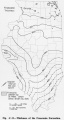
- ...the overlying Ironton Sandstone, and their combined thickness is shown in figure Є-10. The name "Galesville" is applied as far south as the sandy zone can3 KB (454 words) - 21:25, 28 November 2016
- Figure P-2.jpg|{{file:Figure P-2.jpg}}4 KB (620 words) - 20:33, 1 June 2020
- Figure S-4.jpg|{{file:Figure S-4.jpg}}4 KB (515 words) - 23:56, 4 January 2017
- Figure O-2A.jpg|{{file:Figure O-2A.jpg}}6 KB (814 words) - 18:37, 12 January 2017
- ...n in figure 6, and its spatial relations are indicated diagrammatically in figure 7.4 KB (614 words) - 22:26, 3 January 2017
- ...ven in tables 4 and 5, its spatial relations are shown diagrammatically in figure 8, and radiocarbon dates are listed in table 1. Its character is described4 KB (579 words) - 22:20, 3 January 2017
- Figure O-2F.jpg|{{file:Figure O-2F.jpg}}4 KB (558 words) - 21:19, 14 December 2016
- Figure O-2D.jpg|{{file:Figure O-2D.jpg}}5 KB (690 words) - 18:18, 12 January 2017
- Figure P-13.jpg|{{file:Figure P-13.jpg}}4 KB (600 words) - 16:20, 25 January 2017
- ...n in figure 6, and its spatial relations are indicated diagrammatically in figure 7.5 KB (674 words) - 22:07, 12 January 2017
- ...in figure 6, and its spatial relationship is indicated diagrammatically in figure 7.6 KB (833 words) - 22:28, 12 January 2017
- Spatial relations of the Plano Silt Member are shown diagrammatically in figure 8.3 KB (391 words) - 20:51, 12 January 2017
- Figure O-2D.jpg|{{file:Figure O-2D.jpg}}5 KB (691 words) - 21:10, 14 December 2016
- The geographic extent of the Winslow Till Member is shown in figure 6. It is generally less than 20 feet thick.3 KB (414 words) - 22:03, 12 January 2017
- Figure O-2D.jpg|{{file:Figure O-2D.jpg}}4 KB (615 words) - 22:31, 20 December 2016
- Figure D-3A.jpg|{{file:Figure D-3A.jpg}}6 KB (817 words) - 19:34, 22 October 2019
- Figure O-2D.jpg|{{file:Figure O-2D.jpg}}5 KB (759 words) - 17:29, 12 January 2017
- ...is thinner. The geographic extent of the Sterling Till Member is shown in figure 6.3 KB (456 words) - 22:01, 12 January 2017
- ...ther of Wisconsinan deposits from northeastern to west-central Illinois by figure Q-8. ...tion of the dominantly till formations and members is shown in figure Q-5. Figure Q-6 shows graphically the historical development of the time-stratigraphic15 KB (2,213 words) - 16:41, 10 January 2017
- ...the overlying Ironton Sandstone, and their combined thickness is shown in figure Є-10. The name "Galesville" is applied as far south as the sandy zone can4 KB (525 words) - 22:45, 11 January 2017
- Its spatial relations are shown in figure 8.5 KB (755 words) - 15:47, 18 November 2016
- ...) thick and lies in the depth interval of 72.1 to 79.1 ft (22.0 to 24.1 m; Figure 4-70). ...ll Coal (Figure 4-61). A section from the Burning Star No. 4 surface mine (Figure 4-71) also shows nonfissile mudstone beneath the Percy, suggesting paleosol8 KB (1,107 words) - 16:39, 9 February 2022
- ...s less than 20 feet thick. The geographic extent of the member is shown in figure 6.3 KB (488 words) - 22:08, 12 January 2017
- Figure D-3B.jpg|{{file:Figure D-3B.jpg}}6 KB (837 words) - 21:25, 22 October 2019
- ...n Nelson of the ISGS logged the core in 2008. As shown on the graphic log (Figure 4-69), the Bucktown is 3.7 ft (1.13 m) thick and occurs in the depth range Direct comparison of the Bucktown reference core (Figure 4-69) with the Briar Hill reference sections (Figures 4-61 and 4-67) demons7 KB (1,034 words) - 16:39, 9 February 2022
- Figure Q-1A.jpg|{{file:Figure Q-1A.jpg}} Figure Q-1B.jpg|{{file:Figure Q-1B.jpg}}14 KB (2,141 words) - 16:42, 10 January 2017
- ...ven in tables 4 and 5, its spatial relations are shown diagrammatically in figure 8, and radiocarbon dates are listed in table 1. Its character is described5 KB (644 words) - 20:41, 12 January 2017
- ...in the Glasford Formation. This relationship is shown diagrammatically in figure 7.<br>4 KB (520 words) - 22:41, 3 January 2017
- ...ection from the area Wanless mapped in western Illinois is presented here (Figure 4-9). ...n both occupy the second sedimentary cycle underlying the Colchester Coal (Figure 4-9). Fossil spore floras confirm the matchup of the Dekoven and Greenbush7 KB (1,000 words) - 16:31, 9 February 2022
- the map in figure 6.4 KB (599 words) - 07:08, 28 December 2016
- The spatial relations of the Loveland are shown diagrammatically in figure 7. The silts intercalated with the tills of Illinoian age are separately na6 KB (856 words) - 22:23, 3 January 2017
- Its spatial relations are shown in figure 8.6 KB (818 words) - 21:04, 12 January 2017
- ...in the Glasford Formation. This relationship is shown diagrammatically in figure 7.<br>4 KB (582 words) - 22:31, 12 January 2017
- ...The present condition of these exposures is not known. A composite column (Figure 4-9) illustrates the overall relationships. ...(0 to 17 m) thick in Gallatin and Saline Counties, southeastern Illinois (Figure 4-16). The “parting” is largely, but not entirely, sandstone. As mapped8 KB (1,087 words) - 16:30, 9 February 2022
- ...e is thinned by sub-Degonia channels in many more places than are shown in figure M-48. In several areas, sub-Pennsylvanian channels also cut into the Clore.4 KB (490 words) - 16:24, 13 January 2017
- ...ically in figure 7, and the geographic extent of the formation is shown in figure 6. It is the formation underlying the loess in most of the area mapped as I11 KB (1,564 words) - 22:23, 3 January 2017
- The spatial relations are shown diagrammatically by figure 8.4 KB (518 words) - 22:21, 3 January 2017
- The spatial relations of the Loveland are shown diagrammatically in figure 7. The silts intercalated with the tills of Illinoian age are separately na6 KB (911 words) - 21:17, 12 January 2017
- The spatial relations are shown diagrammatically by figure 8.4 KB (584 words) - 20:46, 12 January 2017
- ...graphic form based on field notes made by H.R. Wanless in August of 1929 (Figure 4-17). ...r what Jacobson (1987, 1993) called the “upper split of the Dekoven Coal” (Figure 4-12). As presently recognized, the Abingdon merges with the older Greenbus9 KB (1,279 words) - 16:30, 9 February 2022
- ...ically in figure 7, and the geographic extent of the formation is shown in figure 6. It is the formation underlying the loess in most of the area mapped as I11 KB (1,623 words) - 21:14, 12 January 2017
- ...t 268.0 ft (81.7 m) to the top of the Briar Hill Coal at 323.5 ft (98.6 m; Figure 4-61). Thus, the member is 55.5 ft (16.9 m) thick. ...the Labette Shale in Missouri appears to be correlative to the Big Creek (Figure 4-72).7 KB (1,017 words) - 16:15, 9 February 2022
- ...ick and lies in the depth interval of 566.6 to 568.3 ft (172.7 to 172.3 m; Figure 4-67). The coal is composed of alternating layers of clairain and durain, w ...ore and occurs in the depth interval of 323.5 to 325.0 ft (98.6 to 99.1 m; Figure 4-61).10 KB (1,577 words) - 16:16, 9 February 2022
- ...asper County provides a reference section for the Bevier Coal in Illinois (Figure 4-31). In this core, the Bevier is 1.1 ft (34 cm) thick at a depth of 1,439 ...nd its northward extension but is generally absent from the Western Shelf (Figure 4-34). Its thickness is 1 to 3 ft (30 to 90 cm) in most of the Fairfield Ba8 KB (1,143 words) - 16:36, 9 February 2022
- Figure P-3A.jpg|{{file:Figure P-3A.jpg}} Figure P-3B.jpg|{{file:Figure P-3B.jpg}}24 KB (3,468 words) - 22:19, 19 January 2017
- Figure P-3A.jpg|{{file:Figure P-3A.jpg}} Figure P-3B.jpg|{{file:Figure P-3B.jpg}}24 KB (3,468 words) - 16:01, 20 January 2017
- the idealized sequence shown in figure P-7 is rarely complete, the units that are present have the same relative p Figure P-3A.jpg|{{file:Figure P-3A.jpg}}24 KB (3,539 words) - 16:05, 20 January 2017
- ...from the type Hanover Limestone. However, another version of the section (Figure 4-46) by Van Pelt and Hendricks shows “maybe 20 to 24 feet” (6 to 7 m) ...r is 0.7 ft (21 cm) thick and lies at 352.0 to 352.7 ft (107.3 to 107.5 m; Figure 4-44). The same core is the reference section for the Houchin Creek Coal an12 KB (1,717 words) - 16:17, 9 February 2022
- ...the Davis Coal in the depth interval of 162.0 to 167.5 ft (49.4 to 51.1 m; Figure 4-15). Gamma-ray and electric logs were run in the Morris borehole. ...s the Davis Coal in the depth interval of 174.7 to 176.8 ft (53.2 to 53.9; Figure 4-13).8 KB (1,230 words) - 16:35, 9 February 2022
- ...Gentry (or Gentry’s) Landing on the Ohio River in Hardin County, Illinois (Figure 2-1). Older versions of the Shawneetown 15-minute topographic map locate Ge ...y Rock coal appears considerably higher above the conglomeratic sandstone (Figure 2-1), but if the thinly bedded sandstone above the conglomerate is consider8 KB (1,256 words) - 16:34, 9 February 2022
- ...resented a schematic representation of the “Mazonian delta complex” (their figure 15) showing what appears to be thick peat filling an abandoned distributary A generalized columnar section of the Cardiff area (Figure 4-37) is based on drilling records from the Cardiff Coal Company, circa 1989 KB (1,304 words) - 16:30, 9 February 2022
- Willman and Payne (1942, geologic section 19, p. 295; Figure 4-63). Willman and Payne (1942, geologic section 20, p. 295; Figure 4-63).12 KB (1,630 words) - 16:15, 9 February 2022
- ...and characteristic (fig. M-4). Several conodont assemblage zones, shown in figure M-25, are useful in differentiating Chesterian rocks (Collinson et al., 1977 KB (1,034 words) - 15:54, 13 January 2017
- ...y borehole SDH-306, drilled in sec. 2, T 2 S, R 7 W, Pike County, Indiana (Figure 4-7). ...em (Wanless 1957, geologic section 39, p. 204–205) would have served well (Figure 4-43). Unfortunately, Peppers (1970, p. 50) reported that the section Wanle13 KB (1,879 words) - 16:37, 9 February 2022
- ...c extent of the Banner Formation where it is the surface drift is shown in figure 6, but in the subsurface it is present locally throughout much of western,10 KB (1,522 words) - 22:46, 3 January 2017
- ...and characteristic (fig. M-4). Several conodont assemblage zones, shown in figure M-25, are useful in differentiating Chesterian rocks (Collinson et al., 1977 KB (965 words) - 16:17, 10 January 2017
- ...c extent of the Banner Formation where it is the surface drift is shown in figure 6, but in the subsurface it is present locally throughout much of western,11 KB (1,578 words) - 22:33, 12 January 2017
- ...ea illustrate the relationship of the Colchester Coal to enclosing strata (Figure 4-18). ...0 cm) thick at a depth of 140.6 to 141.6 ft (42.9 to 43.2 m) in this core (Figure 4-19).17 KB (2,555 words) - 16:30, 9 February 2022
- ...thick and lies in the depth range of 352.7 to 359.4 ft (107.5 to 109.5 m; Figure 4-44). This core also serves as a reference section for the Houchin Creek C Extremely high gamma-ray readings are diagnostic (Figure 4-36).10 KB (1,372 words) - 16:17, 9 February 2022
- ...aphic position of coal in the third cyclothem beneath the Colchester Coal (Figure 4-9). Wanless did not raise the point that at some outcrops in western Illi5 KB (713 words) - 16:31, 9 February 2022
- ...ondale into Kentucky; Cumings (1922) did the same for Indiana. As shown by Figure 4-1, numerous authors adjusted the unit boundaries. Some authors ranked the ...o the Davis Coal, currently considered the basal member of the Carbondale (Figure 4-2). Nonetheless, this is a good reference for the Carbondale in western I21 KB (3,121 words) - 16:14, 9 February 2022
- The section illustrated here (Figure 4-25) is from Smith et al. (1970, p. 15). This section illustrates the mult ...in the depth interval of 136.2 to 136.8 ft (41.5 to 41.7 m) in this core (Figure 4-7).15 KB (2,214 words) - 16:29, 9 February 2022
- ...41.5 to 41.7 m) in this core and directly overlies the Mecca Quarry Shale (Figure 4-7).5 KB (719 words) - 16:36, 9 February 2022
- ...and occupies the depth interval from 773.6 to 775.5 ft (235.8 to 236.4 m; Figure 4-78). This core also serves as the reference section for the Energy Shale. ...valent) and underlies the Myrick Station Limestone, a Brereton equivalent (Figure 4-72). First proposed by Wanless (1939), these correlations subsequently ha11 KB (1,593 words) - 16:15, 9 February 2022
- ...the entire core; a graphic log of the relevant portion is presented here (Figure 4-13). ...guish this seam from the Dekoven, which lacks overlying radioactive shale (Figure 4-14).12 KB (1,795 words) - 16:31, 9 February 2022
- ...sburg to be about 15 ft (4.5 m) thick. A graphic section from field notes (Figure 4-58) shows that the base of the Dykersburg was under water at the time the ...ick and lies at the depth interval of 491.9 to 537.9 ft (149.9 to 164.0 m; Figure 4-59).17 KB (2,584 words) - 19:41, 23 August 2023
- ...in the depth interval of 745.4 to 786.0 ft and is 40.6 ft (12.4 m) thick (Figure 4-54). ...Galatia channel” (Nelson et al. 2020). The cross section presented here (Figure 4-55) shows the same relationships.<br>12 KB (1,803 words) - 16:02, 23 August 2023
- Wier (1961). The section (Figure 4-66) leaves much to be desired because it does not position the Antioch re7 KB (940 words) - 16:38, 9 February 2022
- ...comparison of the type and reference sections of the Caseyville Formation (Figure 2-2) raises doubts about the continuity of the unit. The interval between t ...unit labeled “Battery Rock Sandstone” in the type and reference sections (Figure 2-2) actually is the same sandstone, the tectonic subsidence rate must have11 KB (1,561 words) - 16:34, 9 February 2022
- ...ck and occupies the depth interval from 139.4 to 142.6 ft (42.5 to 43.5 m; Figure 4-13).8 KB (1,170 words) - 16:31, 9 February 2022
- ...ld Coal is in the depth range 245.6 to 251.5 ft; the base was not reached (Figure 4-56). The hole was drilled into Peabody Coal Company’s Mine No. 59, wher ...apped two large regions of thick Springfield Coal. The map presented here (Figure 4-57) has been modified from Hatch and Affolter (2002). The larger area cov16 KB (2,297 words) - 16:14, 9 February 2022
- ...in the depth interval of 452 ft 2 in. to 458 ft 10 in. (137.8 to 139.9 m; Figure 4-74). ...Within this larger area, the thickest coal borders the Walshville channel (Figure 4-75). Here, the Herrin is thicker than 8 ft (2.4 m) in large areas and loc18 KB (2,748 words) - 16:35, 9 February 2022
- ...and occupies the depth interval from 775.5 to 785.5 ft (236.4 to 239.4 m; Figure 4-78). As added value, the core contains the Herrin Coal and nearly all the ...the Herrin Coal and beneath the Anna Shale and Brereton Limestone Members (Figure 4-78). Where the Energy Shale is thick, the Anna, Brereton, and younger mem16 KB (2,370 words) - 16:39, 9 February 2022
- ...cause this section was never published, it is reproduced here graphically (Figure 4-30) and verbally (below):<br> ...of the Survant type section in sec. 2, T 2 S, R 7 W, Pike County, Indiana (Figure 4-7). This core exemplifies the Survant Member where its constituent Wheele23 KB (3,526 words) - 16:36, 9 February 2022
- ...Adair 7.5' quadrangle. A graphic version of the section is presented here (Figure 4-21). Wanless described the unit as being 39 ft 6 in. (12.0 m) thick and c ...k and occurs in the depth interval from 264.7 to 303.0 ft (80.7 to 92.4 m; Figure 4-22). The core contains abundant plant fossils.16 KB (2,366 words) - 16:29, 9 February 2022
- ....7 ft (52 cm) thick and occurs in the depth interval from 51.0 to 52.7 ft (Figure 4-60). This core doubles as the type section of the [[Turner Mine Shale Mem9 KB (1,249 words) - 16:16, 9 February 2022
- ...me of their unit boundaries are different from those of Lineback et al. In figure 8, we follow Foster and Colman (1991) for lithostratigraphic unit boundarie15 KB (2,217 words) - 20:19, 22 December 2016
- ...me of their unit boundaries are different from those of Lineback et al. In figure 8, we follow Foster and Colman (1991) for lithostratigraphic unit boundarie15 KB (2,276 words) - 20:48, 22 December 2016
- ....0 ft (99.1 m) to the top of the St. David Limestone at 379.1 ft (115.5 m; Figure 4-61). The Canton is thus 54.1 ft (16.5 m) thick.10 KB (1,407 words) - 16:16, 9 February 2022
- ...) thick and occurs between the depths of 52.7 and 56.7 ft (16.1 to 17.3 m; Figure 4-56).8 KB (1,131 words) - 16:38, 9 February 2022
- ...ction. This is the lower part of Caseyville Formation reference section 3 (Figure 2-2, column 4).9 KB (1,289 words) - 16:34, 9 February 2022
- ...base of Wheeler Coal) to 1,185.3 ft (361.3 m; top of Mecca Quarry Shale) (Figure 4-28). This log represents the situation in most of the Fairfield Basin, wh ...e the Wheeler and Bevier Coals are absent. The log is shown graphically in Figure 4-29.17 KB (2,452 words) - 16:28, 9 February 2022
- ...s Landing below Battery Rock” in Hardin County, Illinois (Lee 1916, p. 15; Figure 2-1). Lee (1916, p. 15–16) created the original description (Figure 2-2). Kosanke et al. (1960) and Nelson (1989) reproduced the section. Geolo54 KB (7,756 words) - 16:31, 9 February 2022
- ...is 3.8 ft (1.16 m) thick at a depth of 136.8 to 140.6 ft (41.7 to 42.9 m; Figure 4-7).11 KB (1,588 words) - 16:29, 9 February 2022


